
White Paper
The Art and Science of the Service-Level Objective
by Theo Schlossnagle
Everyone wants to exceed expectations. This is especially true in the world of Site Reliability Engineering, where whether or not you achieve your goals can be the difference between profit and peril. But what if the goals you are striving to achieve don’t match what it means for the business to be successful? Read this post to understand the art and science of service-level objectives. Among the topics discussed:
- Why setting goals matters, how to design SLOs and how to evaluate their effectiveness
- How histograms can condense massive amounts of information into digestible and actionable insights
- What it means to look at SLOs ‘upside down”

You can’t meet or exceed expectations if no one agrees what the expectations are. In every job, you must understand your objectives to measure your success. In this chapter, we learn what it looks like when an SRE sets goals.
Why set goals?
The main objective of an SRE is to maintain the reliability of systems. Service-Level Objectives (SLOs) are the primary mechanism used by SREs to determine success in this objective. I’m sure you can see that it is difficult to “do your job well” without clearly defining “well.” SLOs provide the language we need to define “well.” You might be more familiar with Service-Level Agreements (SLAs), so let’s begin there. SLAs are thought of by some as the heart of darkness, and by others as the light of redemption. Why the disparity? I believe it’s because of how they are defined. They can be defined in a way that enables producers and consumers to level-set their expectations, or they can be tool for despair, false assurances, or exposing one to dangerous financial liability. Let’s not spend too much time in the darkness.
Often times today, the term SLO is used, and for the purposes of this text, an SLA is simply an SLO that two or more parties have “agreed” to. SLO and SLA are used fairly interchangeably herein, but we make an effort to consider SLAs as “external” multiparty agreements and SLOs as “internal” single-party goals.
Although the concept of an SLA is quite generic and it simply outlines in clear terms how a service will be delivered to a consumer, at least in the world of computing, they tend to focus on two specific criteria: availability and quality of service (QoS). Now, QoS can and should mean different things depending on the type of service. Note that producer and consumer ultimately means business and customer, respectively, but oftentimes, as we define the SLO between components in an architecture, it can mean producing component and consuming component. Examples of a producing component would be a network accessible block storage system and an authorization microservice API; each would have many disparate customers and make promises to those other services about availability, performance, and sometimes even safety.
SLAs are actually quite simple in that you aim to limit your risk by not over- promising and appeal to customers by providing assurances that make them feel comfortable consuming your services. The devil is in the details; while the concept is straightforward, there is art in choosing what to promise and science in quantifying how to promise it.
In an SLA, you’re always promising something over time. This time is often monthly, sometimes daily. The time period over which you promise tends to align with your standard billing cycles but matches your refund policy perfectly. This last part is important. If you are promising something over the course of a day and fail to deliver, you are likely going to back up that promise with a refund for that day’s service. The implications are quite clear when that promise is for a month.
Obviously, many SLAs use multiple time windows to provide a balance between exposure and assurance. For example, if the SLA is violated for one minute in a given day, that day will be refunded, and if the SLA is violated for one hour in a given month, the entire bill for that month is forfeit. I will talk no more of the ramifications of SLA violation in terms of refunds, but instead of just violation. How you choose to recompense for a broken promise is out of the scope of this book; good luck.
The takeaway here is that SLAs make sense only when considered in fixed timeframes, which are called assurance windows. Given how services are trending today and how major service providers disclose their outages (a simplified term for SLA violations), I’ll assume that we use a daily context. All the concepts herein can be applied if that window is different, but do the math and understand your exposure when changing that assurance window.
Now, let’s look at this in context instead of the abstract. I’ll tackle availability before QoS because that’s easier to reason about.
Availability
Availability simply means that your service is available to consume. It functions in only the most basic sense of the word. It does not mean that consumers get the answers they expect when they expect them. I’ll give a few examples of availability that might help illustrate the point.
If you send a package via a major carrier, I would consider it available if the driver comes and picks up your package and it is delivered to the destination. The driver could show up late to pick it up, the contents could be exposed to extreme temperature and thus be damaged, and it could show up three weeks later instead of two days, as requested. It’s available, but utterly unsatisfying. Imagine for a moment the opposite assurance: your package would be delivered on time in pristine condition every time it shipped, but the carrier never showed up to take the package. Now we have perfect QoS, but an utterly unsatisfying experience because it is unavailable.
Availability in computing systems seems like it would be simple to quantify, but there are many different ways to measure availability, and if you articulate them incorrectly, you are either exposed horribly or effectively promising nothing to the consumer. The latter might sound great, but you’ll eventually face the music: higher standards lead to success and consumers are smart.
The most common ways to measure availability are the marking of time quanta or counting failures. The classic SLA language of “99.9% uptime” can put into these terms.
Time Quanta
The idea of time quanta is to take your assurance window (one day) and split it up into pieces. If we were to choose minutes, we’d end up with 1,440 time quanta in that day (unless it is a daylight savings time shift that leads you to question why you work in this field and how, given our bad ideas, humans are still alive at all).
Within each of those time quanta, you can measure for failure. If any failures are detected, the specific time quantum is marked as bad. At the end of the day, your availability is simply the unmarked (good) time quanta over the total (1,440): 1,439/1,440 = 99.930% and 1,438/1,440 = 99.861%. So, with a 99.9% uptime guarantee, you are allowed one minute of down time in that day, but two and you’ve violated your SLA.
This seems simple enough, but it has some flaws that can expose you unnecessarily or provide no acceptable assurance to your consumers—or both. I’m going to use an API service to articulate how this is. Let’s assume that we have a shipping-calculator API service that takes package weight, source, and destination postal code and provides a price.
If we do 100 million transactions per day, that would average to almost 70,000 per minute. If we failed to service one each minute, we’d violate every time quantum of our SLA and have 100% downtime. At the same time, we’ve only failed 1,440 out of 100 million transaction which is a success rate of 99.998%. Unfair!
On the flipside of this, if the consumers really use the app only between 10 AM and 10:30 AM when they’re scheduling all of their packages for delivery, we fail every single transaction from 10:20 to 10:21 and still meet our SLA. From the customer perspective this is doubly bad. First, we’ve met our SLA and disappointed more consumers (3,333,333 failed transactions versus 1,440) and we’ve had an effective uptime of one minute out of the 30 that is important to them; a perceived uptime of only 96.666%.
If your usage is spread evenly throughout the day, this approach can work and be simple to understand. Most services do not have an even distribution of transactions throughout a day, and, while simplicity is fantastic in SLAs, this method is too flawed to use.
Transactions
Another common method is to use the raw transactions themselves. Over the course of our assurance window, we simply need to count all of the attempted transactions and the number successfully performed. In many ways, this provides a much stronger assurance to a client because it clearly articulates the probability for which they should expect to receive service.
Following the earlier example, if we have 100 million transactions and have a 99.9% uptime guarantee, we can fail to service 100,000 without breaking our SLA. Keep in mind that this might sound like a lot, but at an average 70,000 per minute, that is identical to a continuous two-minute outage resulting in an SLA violation. The big advantage should be obvious; it allows us to absorb aberrant behavior that affects a very small set of consumers over the course of our entire assurance window without violating the SLA (mutual best interest).
One significant challenge is that it requires you to be able to measure attempted transactions. In the network realm, this is impossible: if packets don’t show up, how would we know they were ever sent? Regarding online services, they are all connected by a network that could potentially fail. This means that it is impossible for us to actually measure attempted transactions. Wow. So, even though this is clearly an elegant solution, it allows for too much deniability on the part of the producer to provide strong assurances to the consumer. How can we fix this?
Transactions Over Time Quanta
The best marriages expose the strengths of the partners and compensate for their weaknesses. This is certainly the case for the marriage of the previous two approaches. I like to call this “Quantiles over Quantums” just because it sounds catchy.
By reintroducing the time quantum into transactional analysis, we compromise in the true sense of the word. We remove the fatal flaw of transactional quantification in that if the “system is down” and attempted transactions cannot even be counted, we can mark a quantum as failed. This tightly bounds the transaction methods fatal flaw. On the flip side, the elegance of the transactional method allowing insignificant failures throughout the entire assurance window is reduced in effectiveness (precisely by the number of time quanta in the assurance window).
Now, in our previous example of 100 million transactions per day, instead of allowing for up to 100,000 failures throughout the day, we now have an additional constraint that can’t have more than 69 per minute (assuming that we preserve the 99.9% to apply to the time quantum transaction assurance).
The articulation of this SLA would be as follows:
The service will be available and accept requests 99.9% of the minutes (1,439 of 1,440) of each day. Availability is measured each minute and is achieved by servicing a minimum of 99.9% of the attempted transactions. If a system outage (within our control) causes the inability to measure attempted transaction, the minute is considered unavailable.
All of this is just a balancing act; this is the art of SLAs. Although it is more difficult to achieve this SLA, when you do miss, you can feasibly make statements like, “We were in violation for eight minutes,” instead of, “We violated the SLA for Wednesday.” Calling an entire day a failure is bad for business and bad for morale. SLAs do a lot to inspire confidence in consumers, but don’t forget they also serve to inspire staff to deliver amazing service.
For many years, we’ve established that “down” doesn’t mean “unavailable.” The mantra “slow is the new down” is very apt. Most good SLAs now consider service times slower than a specific threshold to be “in violation.” All of the previously discussed methods still apply, but a second parameter dictating “too slow” is required.
On Evaluating SLOs
The first and most important rule of improving anything is that you cannot improve what you cannot measure; at least you cannot show that you’ve improved it.
We’ve talked about the premise of how SLOs should be designed. I’m in the “Quantiles of Quantums” camp of SLO design because I think it fairly balances risk. The challenge is how to quantitatively set SLOs. SLAs are data-driven measurements, and the formation of an SLO should be an objective, data-driven exercise, as well. Too often, I see percentiles and thresholds plucked from thin air (or less savory places) and aggressively managed to; this is fundamentally flawed.
It turns out that quite a bit of math (and largely statistics) is required to really understand and guide SLOs; too much math, in fact, to dive into in a single overview chapter. That said, I’ll try to give the tersest summary of the required math.
First, a Probability Density Function (PDF) is a function that takes a measurement as input and a probability that a given sample has that measurement as an output. In our systems these “functions” are really empirical sets of measurements. As an example, if I took the latency of 100,000 API requests against and endpoint, I could use that data to answer an estimation to the question: “What’s the probability that the next request will have a latency of 1.2 ms?” The PDF answers that question.
A close dancing partner of the PDF is the Cumulative Density Function (CDF). It is simply the integral (hence the name cumulative) of the PDF. The CDF can answer the question: “What’s the probability that the next request will have a latency less than (or greater than) 1.2 ms?”
Probabilities range from 0 (nope) to 1 (certainly), just as percentages range from 0% to 100%. Percentiles (like 99th percentile) use percentages as their terms; “quantiles” are the same thing, but they use probabilities as their terms. The 99th percentile is the 0.99 quantile or q(0.99). The quantile function is simply a mapping to the CDF; in a typical graph representation of a CDF, we ask what is the x-axis value when the y-axis value is 0.99? In Figure 21-1, q(0.99) (or the 99th percentile) is about 270.
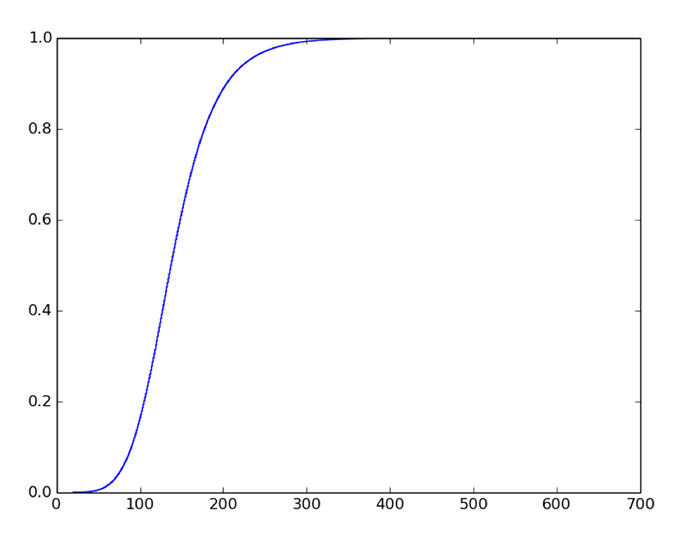
Figure 21-1. CDF function. 0.99 (y-axis) 270 (x-axis)
Oftentimes in computing, you’ll hear normal or Pareto or gamma distributions, which are different mathematical models that indicate how you expect your measurement samples to be distributed (Figure 21-2). The hard truth is that you will almost never see a normal distribution from a real-world computing system; it just doesn’t happen. Things sometimes look like gamma distributions, but computers and systems of computers are complex systems and most sample distributions are actually a composition of several different distribution models. More important, your model is often less important than the actual data.
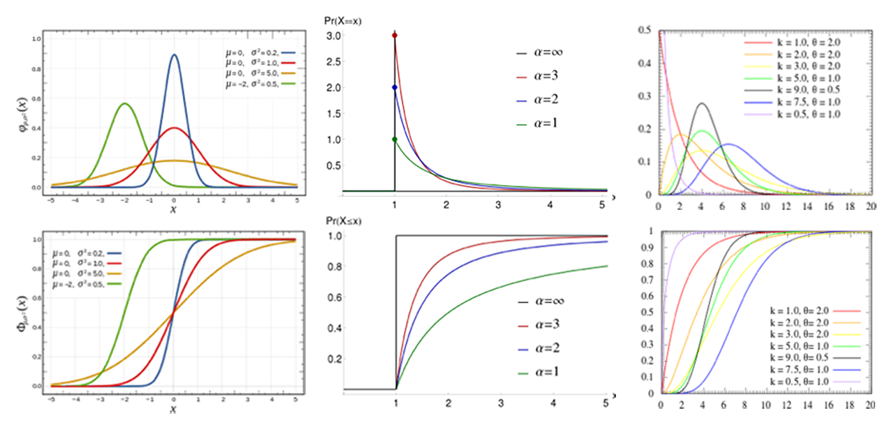
Fig. 21-2. Common PDFs and CDFs
Pareto distributions model things like hard disk error rates and file size distributions. In my experience, because slow is also considered down, most SLAs and SLOs are articulated in terms of latency expectations. We track the latencies on services to both inform the definition of external SLAs as well as assess our performance to our internal SLOs.
Histograms
Histograms allow us to compress a wealth of dense information (latency measurements) into a reasonably small amount of space informationally while maintaining the ability to interrogate important aspects of the distribution of data (such as approximating quantile values).
In Figure 21-3, we see what represents the seconds of latency under real-world usage. The x-axis is in seconds, so the measurements of 1.0 m and 1.5 m are (in milli-units, in this case milliseconds). The y-axis represents the number of samples. The area of each bar represents a set of samples that fall into the latency range depicted by boundaries of the bar on x-axis. Just underneath the x-axis, we can see markers indicating “quantile boxing” showing the q(0) (the minimum), q(0.25) (the 25th percentile), q(0.5) (the median), and q(0.75) (the 75th percentile). The q(1) (the maximum) isn’t visible on the graph as much of the long tail of the distribution is outside the right side of the viewport of the graph. The vertical line (m) indicates the arithmetic average (mean) of the distribution. The above graph packs a punch! There’s a wealth of information in there.
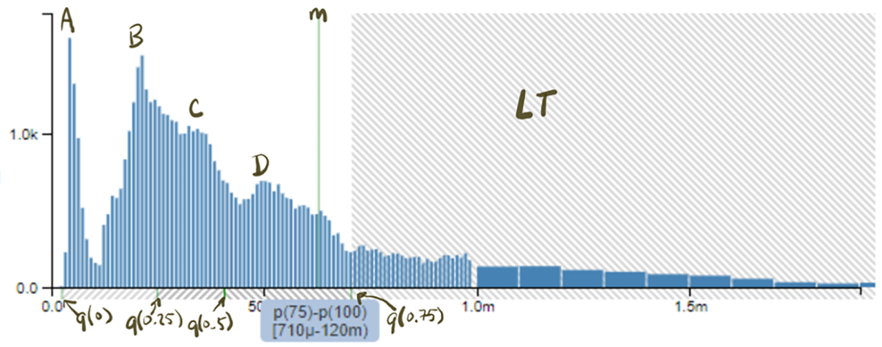
Figure 21-3. An example latency histogram for data service requests
On the left side of the histogram, we see a spike (A) called a mode that represents services that were served fast (likely entirely from cache) and the distribution between (A) and 1.0 ms looks comprised of several different behaviors (B), (C), and (D). If you refer to the gamma distribution PDF graph, this looks a bit like several of those graphs stacked atop one another. The largest samples in this histogram are actually “off the graph” to the right in part of the distribution’s long tail (LT), but the blue underbox indicates that p(100) (our “maximum”) is 120 ms. It’s important to recognize that most real-world distributions have complex cumulative patterns and long tail-distributions making simple statistical aggregates like min, max, median, average, and so on result in a poor understanding of the underlying data.
Given the data that is used to draw this histogram (bins and sample counts) we can estimate arbitrary quantiles (and inverse quantiles) and more advanced characteristics of the workload such as modal cardinality (the number of bumps in a histogram).
In addition to some typical 99th percentile SLA, we might also want to establish internal SLOs that state 75% or more of the requests against this service should complete in 1 ms or less. The histogram in Figure 21-3 happens to comprise samples over a 1-second period and contains more than 60,000 samples. If you’ve been looking at “averages” (which happens to be vertical indicator line) of your data over time, this visualization of one second’s worth of data should be a wake-up call to the reality of your system behavior.
The more challenging question in setting an SLO around this service is “how fast should it be for most consumers?” The graph should inform us whether we’re succeeding, but the business and technical requirements around the service should be the driver for the answer to that question. In this particular case, this is a data- retrieval API and the applications that it powers have negotiated that 99% of the requests they make should be services within 5 ms. Doing analysis on the data, the previous example has a q(0.99) = 3.37 ms. Yay!
Where Percentiles Fall Down (and Histograms Step Up)
Knowing that our q(0.99) is 3.37 ms, we’re currently “exceeding” our SLO of 5 ms at 99%. But, how close are we to the edge? A percentile grants no insight to this. The first sample slower than the 99th percentile sample could be 10 ms or (more likely) could be less than 5 ms; yet, we don’t know. Also, we don’t know what percentage of our consumers are suffering from “slow” performance.
Enter the power of histograms, given the whole histogram to work with, we can actually count the precise number of samples that exceeded our 5-ms contract. Although you can’t tell from the visualization alone, with the underlying data we can calculate that 99.4597% of the population is faster than 5 ms, leaving 0.5403% with unsatisfying service; 324 of our roughly 60,000 samples. Further, we can investigate the distribution and sprawl of those “outlier” samples. This is the power of going beyond averages, minimum, maximums, and even arbitrary percentiles. You cannot understand the true behavior of your systems and think intelligently about them without measuring how they behave. Histograms are perhaps the single most powerful tool in your arsenal.
Parting Thought: Looking at SLOs upside down
As an industry, we have arbitrarily selected both the percentile and the performance for which we set our SLOs. There should be more reason to it than that. If you are measuring at q(0.99), is that really because it is satisfactory that 1% of your consumers can receive a substandard experience? This is something to think about and debate within your team and organization as a whole.
It has also been standard to measure a specific quantile and construct the SLO around the latency at that specific quantile. Here is where I believe the industry might consider looking at this problem upside down. What is special about that 1% of consumers that they can receive worse than desirable performance? Would it be better if it were 0.5% or 0.1%? Of course it would. Now, what is special about your performance criteria? Is it the 5 ms in our data retrieval example (or perhaps 250 ms in a user experience example)? Would it be better if it were faster? The answer to this is not so obvious? Who would notice?
Given this, instead of establishing SLOs around the q(0.99) latency, we should be establishing SLOs around 5ms and analyze the inverse quantile: q–1(5 ms)? The output of this function is much more insightful. The first just tells us how slow the 99th percentile is, the latter indicates what percentage of the population is meeting or exceeding our performance target.
Ultimately, SLOs should align with how you and your potential consumers would expect the service to behave. SLOs are simply the precise way you and your team can articulate these expectations. Make SLOs match you, your services, and your customers; another organization’s SLOs likely make no sense at all for you.
Another advantage of SLOs is that by exceeding your SLOs they quantitatively play into your budgets for taking risk. When you’re close to violating an SLO, you turn the risk dial down; if you have a lot of headroom, turn the risk dial up and move faster or innovate!